Gallery 2: Profile Plots

This page provides example on how to plot 3D TUFLOW FV results as a function of depth (a 3D vertical profile). This notebook is used in combination with the TUFLOW FV Python Toolbox (tfv) package. To follow along on your own computer, please download the demonstration notebooks from the TUFLOW Downloads Page. Look for the TUFLOW FV Python Toolbox download. Installation instructions are provided on our TUFLOW FV Python Toolbox Wiki Page.

import xarray as xr  # We utilise xarray to do all the heavy lifting 
import numpy as np
import tfv.xarray
from pathlib import Path # We'll also make use of the `pathlib` module to assist with managing file-paths, although this is entirely optional! 
import matplotlib.pyplot as plt

Open TUFLOW FV Model Result

model_folder = Path(r'..\..\data')
model_file = 'HYD_002.nc'

fv = xr.open_dataset(model_folder / model_file, decode_times=False).tfv

Define Locations for Extraction

locs = {
    'P1' : (159.0758, -31.3638),
    'P2' : (159.0845,  -31.3727),
    'P3' : (159.0906,  -31.3814),
    'P4' : (159.1001,  -31.3948),
    'P5' : (159.1154,  -31.4032),
    'P6' : (159.1266,  -31.4105),
    'P7' : (159.1202,  -31.4165),
    'P8' : (159.1178,  -31.4236),
    'P9' : (159.1277,  -31.4402)
}

loc = 'P1'

Extract Profile Data Directly from TUFLOW FV Xarray Accessor Object

prof = fv.get_profile(locs[loc],variables=['V','TEMP','SAL'])
#prof.head() # Uncomment to review the data array 

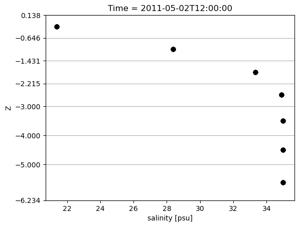
Plot Profile

time = '2011-05-02 12:00'
prof.sel(Time=time).plot.scatter(x='SAL',y='Z', color='black', lw=1)

# Show layerfaces
zfaces = prof['layerface_Z'].sel(Time=time)
plt.yticks(zfaces)
plt.grid(axis='y')
plt.show()

This concludes the examples on profile plotting.