Gallery 1: Timeseries Plots

This notebook provides a series of timeseries examples used in combination with the TUFLOW FV Python Toolbox (tfv) package. To follow along on your own computer, please download the demonstration notebooks from the TUFLOW Downloads Page. Look for the TUFLOW FV Python Toolbox download. Installation instructions are provided on our TUFLOW FV Python Toolbox Wiki Page.

import xarray as xr  # We utilise xarray to do all the heavy lifting 
import tfv.xarray
from pathlib import Path # We'll also make use of the `pathlib` module to assist with managing file-paths, although this is entirely optional! 
import matplotlib.pyplot as plt

Open TUFLOW FV Model Result

model_folder = Path(r'..\..\data')
model_file = 'HYD_002.nc'

fv = xr.open_dataset(model_folder / model_file, decode_times=False).tfv
#fv  # Uncomment this to display the data variables

Extract Time Series Data

locs = {
    'P1' : (159.0758, -31.3638),
    'P2' : (159.0845,  -31.3727),
    'P3' : (159.0906,  -31.3814),
    'P4' : (159.1001,  -31.3948),
    'P5' : (159.1154,  -31.4032),
    'P6' : (159.1266,  -31.4105),
    'P7' : (159.1202,  -31.4165),
    'P8' : (159.1178,  -31.4236),
}

ts = fv.get_timeseries(['H', 'V', 'TEMP'],locs)
#ts  # Uncomment this to display the data variables

Extracting timeseries, please wait: 100%|████████████████████████████████████████████| 145/145 [00:01<00:00, 87.48it/s]

Plot Single Time Series

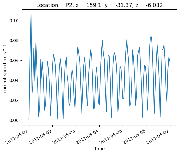
Plot the depth averaged velocity at the point P2.

ts['V'].sel(Location='P2').plot()

[<matplotlib.lines.Line2D at 0x277a513c1d0>]

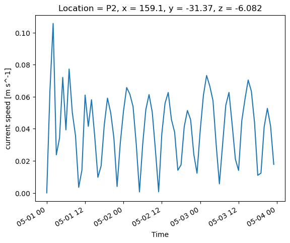
Trim the Time to Plot

ts['V'].sel(Time=slice('2011-05-01','2011-05-03'), Location='P2').plot()

[<matplotlib.lines.Line2D at 0x277a796a710>]

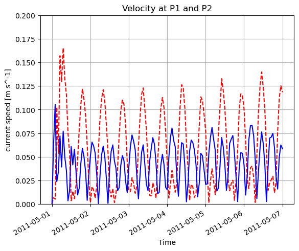
Plot Time Series at Multiple Locations

# Plot the time series 
ts['V'].sel(Location='P1').plot(color='red', linestyle='--')
ts['V'].sel(Location='P2').plot(color='blue')

# Tidy up the plot
plt.title('Velocity at P1 and P2')
plt.grid()
plt.ylim(0,0.2)
plt.show()

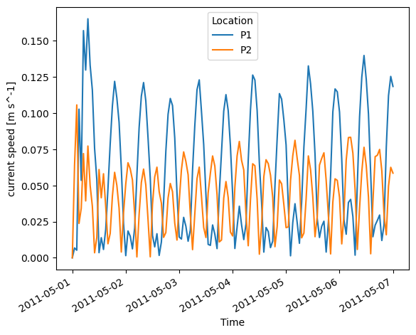
# Or you can try this for something quick
ts['V'].sel(Location=['P1','P2']).plot.line(x='Time', hue='Location')

[<matplotlib.lines.Line2D at 0x277a7ce7f50>,
 <matplotlib.lines.Line2D at 0x277a7cf8390>]

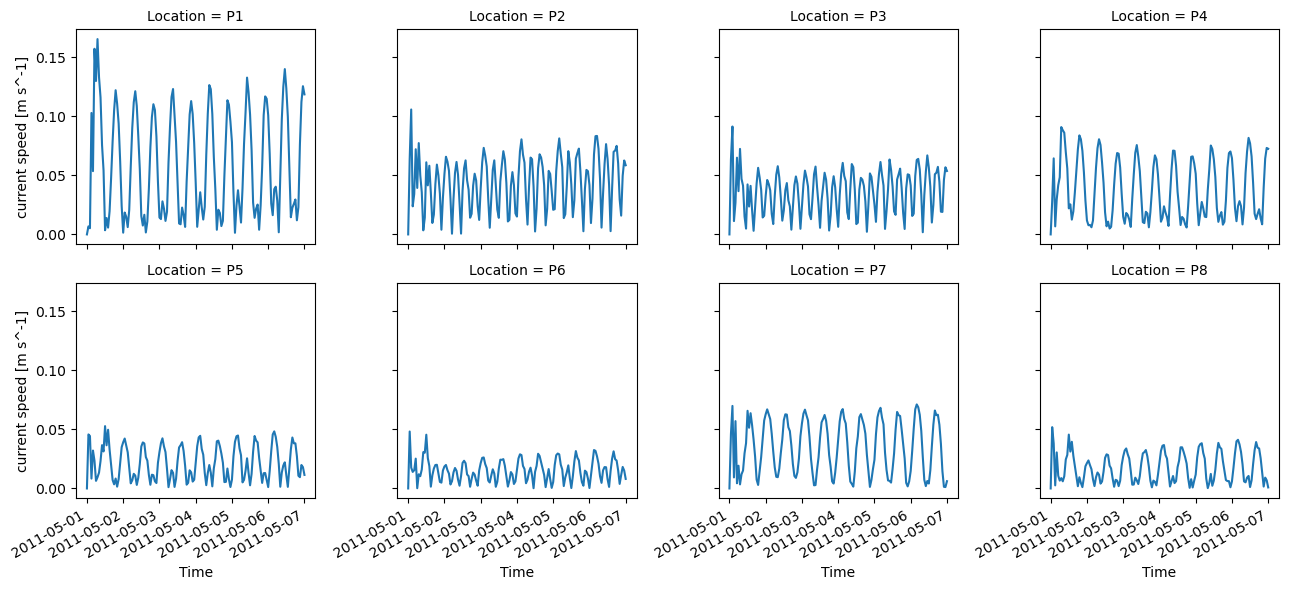
Plot Time Series at All Locations

ts['V'].plot.line(x='Time', col='Location',col_wrap=4)

<xarray.plot.facetgrid.FacetGrid at 0x277a7d07d90>

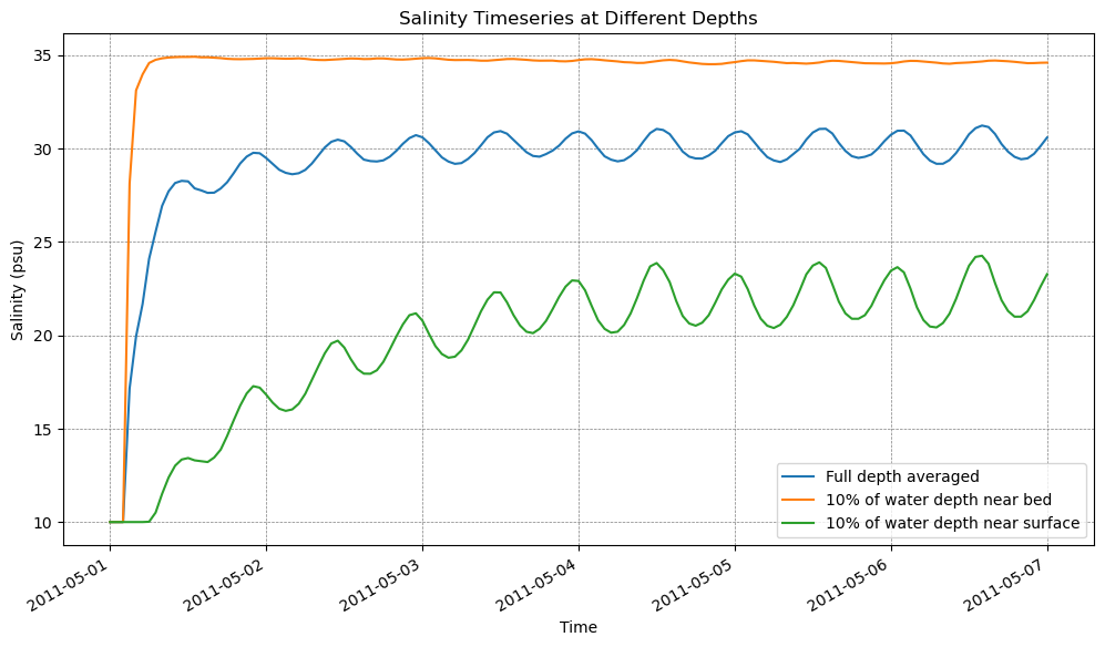
Plot Times Series at Multiple Depths and Save to Disk

# Extract the data at different depths (see also height, elevation and depth datum methods)
ts_dave = fv.get_timeseries(['V', 'TEMP','SAL'],locs,datum='sigma',limits=(0,1))  #   Full depth averaged
ts_bot_10pct = fv.get_timeseries(['V', 'TEMP','SAL'],locs,datum='sigma',limits=(0,0.1))  # 10% of water depth near bed
ts_top_10pct = fv.get_timeseries(['V', 'TEMP','SAL'],locs,datum='sigma',limits=(0.9,1))  # 10% of water depth near surface

Extracting timeseries, please wait: 100%|████████████████████████████████████████████| 145/145 [00:01<00:00, 81.87it/s]
Extracting timeseries, please wait: 100%|████████████████████████████████████████████| 145/145 [00:01<00:00, 92.42it/s]
Extracting timeseries, please wait: 100%|████████████████████████████████████████████| 145/145 [00:01<00:00, 91.38it/s]

# Plot the salinity timeseries in three colours on a plot
fig, ax = plt.subplots(figsize=(12,6))
ts_dave['SAL'].sel(Location='P2').plot(ax=ax, label='Full depth averaged')
ts_bot_10pct['SAL'].sel(Location='P2').plot(ax=ax, label='10% of water depth near bed')
ts_top_10pct['SAL'].sel(Location='P2').plot(ax=ax, label='10% of water depth near surface')

ax.legend()
ax.set_ylabel('Salinity (psu)')
ax.set_xlabel('Time')
ax.set_title('Salinity Timeseries at Different Depths')
ax.grid(color='grey', linestyle='--', linewidth=0.5)

plt.show()

# Save the plot to a jpg file
fig.savefig(Path('./plots') / 'salinity_timeseries.jpg', dpi=300)

Convert to Pandas Dataframe

ts_df = ts.to_dataframe()
# ts_df.head()  # Uncomment if you'd like to see a description of the pandas DataFrame

This concludes the examples on time series plotting.