Example 1. Basic usage with the TfvDomain Xarray accessor
This notebook provides a high-level view on the typical usage of the TfvDomain xarray accessor tool.
To try this out for yourself, you can get a copy of the TUFLOW FV tutorial model result file from here:
import xarray as xr  # We utilise xarray to do all the heavy lifting
import tfv.xarray
Loading data
We treat TUFLOW FV netcdf files like any ordinary xarray dataset.
Older copies of TUFLOW FV do not have a cf-compliant datetime, so you need to add in the kwarg argument decode_times=False so that xarray doesn’t try to convert the time array into a datetime array.
The standard Xarray print output for a TUFLOW FV isn’t very easy or useful because of the large number of variables and coordinates. Also, native xarray isn’t able to help us process these files in any standard manner because they are unstructured.
ds = xr.open_dataset("../HYD_002_extended.nc", decode_times=False)
ds
<xarray.Dataset>
Dimensions:              (Time: 145, NumCells2D: 1375, MaxNumCellVert: 4,
                          NumCells3D: 6453, NumVert2D: 1419,
                          NumLayerFaces3D: 7828, Sum2DVertCells: 5285)
Dimensions without coordinates: Time, NumCells2D, MaxNumCellVert, NumCells3D,
                                NumVert2D, NumLayerFaces3D, Sum2DVertCells
Data variables: (12/26)
    ResTime              (Time) float64 1.848e+05 1.848e+05 ... 1.85e+05
    cell_Nvert           (NumCells2D) int32 4 4 4 4 4 4 4 4 ... 4 4 4 4 4 4 4 4
    cell_node            (NumCells2D, MaxNumCellVert) int32 3 1 2 ... 1414 1416
    NL                   (NumCells2D) int32 6 5 10 5 10 9 6 10 ... 5 7 6 7 5 7 7
    idx2                 (NumCells3D) int32 1 1 1 1 1 ... 1375 1375 1375 1375
    idx3                 (NumCells2D) int32 1 7 12 22 27 ... 6428 6435 6440 6447
    ...                   ...
    TEMP                 (Time, NumCells3D) float32 ...
    SAL                  (Time, NumCells3D) float32 ...
    RHOW                 (Time, NumCells3D) float32 ...
    node_NVC2            (NumVert2D) int32 1 2 2 2 4 2 2 4 4 ... 4 2 4 1 4 2 2 2
    node_cell2d_idx      (Sum2DVertCells) int32 1 1 2 1 ... 1373 1375 1374 1375
    node_cell2d_weights  (Sum2DVertCells) float64 1.0 0.4657 ... 0.4836 0.5164
Attributes:
    Origin:     Created by TUFLOWFV
    Type:       Cell-centred TUFLOWFV output
    spherical:  true
Dry depth: 0.01This is where the tfv.xarray module steps in, to enhance the functionality of native xarray to enable working with unstructured files (currently only supporting TUFLOW FV outputs).
There are two ways to enable the extension.
Calling the appropriate accessor method on the dataset, e.g.,
fv = tfv.xarray.TfvDomain(ds)
(we are using a TUFLOW FV domain file, or in other words, a 2D / 3D spatial netcdf)Simplying calling
fv = ds.tfvwhich will attempt to auto-detect what you have. This usually works.
# These are equivalent - use whichever you prefer.
fv = ds.tfv
# fv = tfv.xarray.TfvDomain(ds)
fv
<xarray.Dataset>
Dimensions:      (Time: 145, NumLayerFaces3D: 7828, NumCells2D: 1375,
                  NumCells3D: 6453)
Coordinates:
  * Time         (Time) datetime64[ns] 2011-02-01 ... 2011-02-07T00:00:11.899...
Dimensions without coordinates: NumLayerFaces3D, NumCells2D, NumCells3D
Data variables:
    ResTime      (Time) float64 1.848e+05 1.848e+05 ... 1.85e+05 1.85e+05
    layerface_Z  (Time, NumLayerFaces3D) float32 ...
    stat         (Time, NumCells2D) int32 ...
    H            (Time, NumCells2D) float32 ...
    V_x          (Time, NumCells3D) float32 ...
    V_y          (Time, NumCells3D) float32 ...
    D            (Time, NumCells2D) float32 ...
    ZB           (Time, NumCells2D) float32 ...
    TEMP         (Time, NumCells3D) float32 ...
    SAL          (Time, NumCells3D) float32 ...
    RHOW         (Time, NumCells3D) float32 ...
Attributes:
    Origin:     Created by TUFLOWFV
    Type:       Cell-centred TUFLOWFV output
    spherical:  true
Dry depth: 0.01TUFLOW FV domain xarray accessor object
As you can see, the print output is now shorter, and only shows the “useful” variables. All the original data is still there, but has just been hidden in this print view.
You can also see that the the Time coordinate is based on a properly formatted datetime array.
Conceptually - this TfvDomain object has just added on a bunch useful methods to help you work with the TUFLOW FV unstructured data.
All the hard work is being done behind the scenes by the existing tools available in FvExtractor, or the plotting functions in Visual.
Some Common Use Examples
Spatial Plots
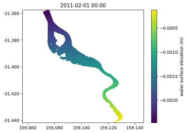
By default, the tool will plot the first variable it finds, with the first timestep it finds.
For many model results, this will be surface elevation at the first timestep.
fv.plot()
<tfv.visual.SheetPatch at 0x176448a60>
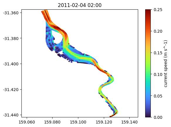
You can add lots of arguments to style plots to your liking.
There is also some magic behind the scenes - if you have V_x and V_y in your dataset, you can request V or VDir directly.
fv.plot('V', '2011-02-04 02:00', cmap='turbo', clim=(0, 0.25), datum='depth')

# Other things to try:
# Depth-averaging, e.g., datum=["sigma", "height", "depth"], combined with limits
# Shading = ["interp", "patch", "contour"]

# Time can be provided as a str, a Timestamp object, or a simple integer.
<tfv.visual.SheetPatch at 0x16b32f6a0>
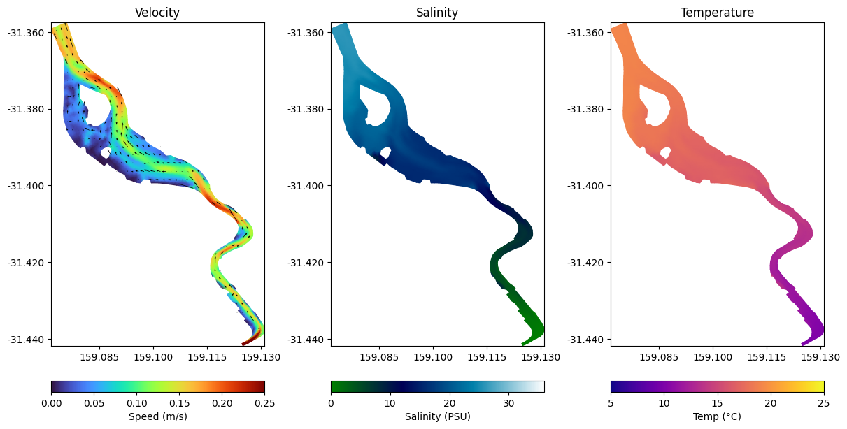
All the plotting methods can be embedded in normal matplotlib figures, so you can create complex plots.
Here is a very simple example and which provides some building blocks you might use.
import matplotlib.pyplot as plt

# With datum='depth', this is the surface 1m.
# experiment with datum='height' to see how the results change.
datum = 'depth'
limits = (0,1)

fig, axes = plt.subplots(ncols=3, figsize=(12, 6), constrained_layout=True)

ts = '2011-02-05 02:00'

ax = axes[0]
p1 = fv.plot('V', ts, ax=ax,  shading='interp', cmap='turbo', clim=(0, 0.25), datum=datum, limits=limits, colorbar=False)  # By setting datum to depth, this is now the "surface 1m")
v1 = fv.plot_vector('V', ts, ax=ax, color='k')   # We can plot a vector overlay using the `plot_vector` method here
ax.set_title('Velocity')
plt.colorbar(p1.patch, ax=ax, orientation='horizontal', label='Speed (m/s)')

ax = axes[1]
p2 = fv.plot('SAL', ts, ax=ax,  shading='interp', cmap='ocean', clim=(0, 36), datum=datum, limits=limits, colorbar=False)
ax.set_title('Salinity')
plt.colorbar(p2.patch, ax=ax, orientation='horizontal', label='Salinity (PSU)')

ax = axes[2]
p3 = fv.plot('TEMP', ts, ax=ax, shading='interp', cmap='plasma', clim=(5, 25), datum=datum, limits=limits, colorbar=False)
ax.set_title('Temperature')
plt.colorbar(p3.patch, ax=ax, orientation='horizontal', label='Temp (°C)')

plt.show()
Interactive Plotting
The tfv tools work great in interactive python, such as with Jupyterlab.
Often we jsut want to interactively look at our model results to ensure that everything is working well, or to understand the results. We can use the plot_interactive method to enable animated plotting so we can dig deeper into the results.
In general, the arguments to the plot_interactive method are the same as the plot method. We can also add on vectors, and setup multiple plots. This is covered in another tutorial.
We first need to turn on interactive plotting by enabling matplotlib in widget model - run this once %matplotlib widget. You may need to install ipympl if this fails.
%matplotlib widget
Output hidden because it doesn’t render nicely in on tutorial page
fv.plot_interactive('V', cmap='turbo', clim=(0,0.5), datum='depth', vectors=True)
plt.show()
Show code cell output
To turn off interactive plotting (which can often make your sessions run faster, a good idea when you don’t need it), use %matplotlib inline
%matplotlib inline
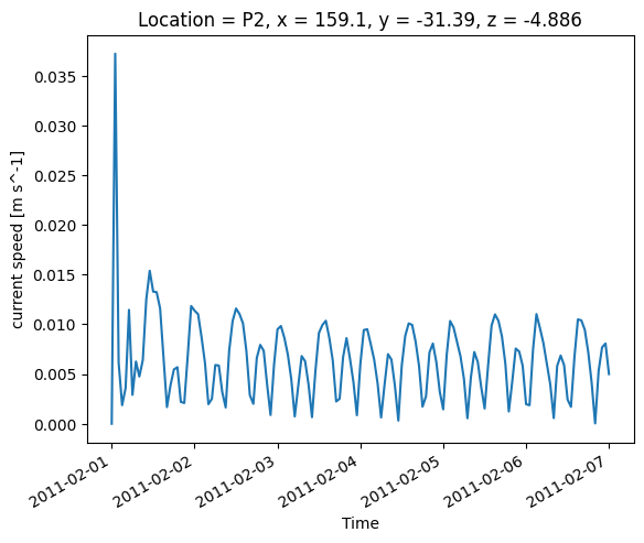
Extracting and plotting timeseries
To grab a timeseries from the model domain result, we can provide either a simple tuple with (X,Y), or a dictionary with some named locations.
For example, we may wish to extract two timeseries at “P1” and “P2”, which we then want to plot and convert to a pandas dataframe.
By default, we’ll always be returned with Xarray objects, but these are easily converted by calling the .to_dataframe() method
locs = {
    'P1': (159.1, -31.39),
    'P2': (159.115, -31.395),
}

ts = fv.get_timeseries(['H', 'V', 'TEMP'], locs)
ts_df = ts.to_dataframe()

# Output hidden because progress bar's don't render nicely here!
Show code cell output
Extracting timeseries, please wait: 100%|███████████████████████████████████████████████████████████████████████████████████████████████████████████████████████████████████████████████████| 145/145 [00:00<00:00, 145.54it/s]
ts
<xarray.Dataset>
Dimensions:   (Time: 145, Location: 2)
Coordinates:
  * Time      (Time) datetime64[ns] 2011-02-01 ... 2011-02-07T00:00:11.899897200
  * Location  (Location) <U2 'P1' 'P2'
    x         (Location) float64 159.1 159.1
    y         (Location) float64 -31.39 -31.39
    z         (Location) float32 -1.068 -4.886
Data variables:
    H         (Time, Location) float64 -0.001545 -0.0008779 ... 0.06717 0.07611
    V         (Time, Location) float64 0.0 0.0 0.05311 ... 0.01978 0.004996
    TEMP      (Time, Location) float64 20.0 20.0 19.96 ... 17.36 16.61 17.34
Attributes:
    Origin:     Timeseries extracted from TUFLOWFV cell-centered output using...
    Type:       Timeseries cell from TUFLOWFV Output
    spherical:  true
    Dry depth:  0.01
    Datum:      sigma
    Limits:     (0, 1)
Agg Fn: meants_df.head()
| x | y | z | H | V | TEMP | ||
|---|---|---|---|---|---|---|---|
| Time | Location | ||||||
| 2011-02-01 00:00:00.000000000 | P1 | 159.100 | -31.390 | -1.067781 | -0.001545 | 0.000000 | 20.000000 |
| P2 | 159.115 | -31.395 | -4.886311 | -0.000878 | 0.000000 | 20.000001 | |
| 2011-02-01 01:00:17.809977600 | P1 | 159.100 | -31.390 | -1.067781 | 0.049078 | 0.053110 | 19.960014 |
| P2 | 159.115 | -31.395 | -4.886311 | 0.108249 | 0.037206 | 19.989328 | |
| 2011-02-01 02:00:00.263494800 | P1 | 159.100 | -31.390 | -1.067781 | -0.091997 | 0.003442 | 19.927108 |
ts['V'][:, 1].plot()
[<matplotlib.lines.Line2D at 0x176473940>]
Sheet Timeseries
Often we want to work in both time and space. TUFLOW FV is often run in a 3D mode, so we need to reduce 3D results to 2D using some dimension reduction logic.
Most often we just depth-average, which is the default throughout the tfv.
The get_sheet method will handle extracting 2D or 3D (to 2D) results, and will take care of the dimension reduction as needed.
You can supply the following arguments to control how the dimensino reduction for 3D variables is handled:
datum: One ofsigma, depth, height, elevationlimits: A tuple containing limits, for example (0, 1) or (5, 10).agg: One ofmean, min, max. This is the general aggregation method to apply to the selected vertical range.
By default, this will bemean(i.e., take the vertically weighted mean over the depth range based ondatumandlimits). Usingmaxwill return the maximum value in our selected depth range, and so on withmin.
For more info, see the TUFLOW FV wiki page
# This grabs ALL timesteps between the 2nd to 4th of Feb 2011, and takes the average of the top 2m
sht = fv.get_sheet('SAL', slice('2011-02-02', '2011-02-04'), datum='depth', limits=(0,2))
sht
<xarray.Dataset>
Dimensions:      (Time: 72, NumLayerFaces3D: 7828, NumCells2D: 1375)
Coordinates:
  * Time         (Time) datetime64[ns] 2011-02-02T00:00:49.390214400 ... 2011...
Dimensions without coordinates: NumLayerFaces3D, NumCells2D
Data variables:
    ResTime      (Time) float64 1.848e+05 1.848e+05 ... 1.849e+05 1.849e+05
    layerface_Z  (Time, NumLayerFaces3D) float32 ...
    stat         (Time, NumCells2D) int32 -1 -1 -1 -1 -1 -1 ... -1 -1 -1 -1 -1
    SAL          (Time, NumCells2D) float64 0.0 0.0 0.0 0.0 ... 28.63 28.83 28.7
Attributes:
    Origin:     Created by TUFLOWFV
    Type:       Cell-centred TUFLOWFV output
    spherical:  true
Dry depth: 0.01TUFLOW FV domain xarray accessor object
This result returned another TfvDomain object - we can plot these 2D results using the .plot method we saw above, or we can now use them for something else (e.g., custom analysis)
Built-in statistics
The tfv tools can handle basic statistics. The get_statistics method basically first calls the get_sheet method above for you, and then also does some statistics.
# List of percentiles to grab, as well as some common stats
stats = ['p5', 'p50', 'p97.5', 'p99', 'min', 'mean', 'max']

# Do stats on velocity for the bottom 1m (default of limits is (0, 1), and with datum='height', we get the bottom 1m).
stat = fv.get_statistics(stats, 'V', datum='height')
stat
<xarray.Dataset>
Dimensions:      (Time: 1, NumLayerFaces3D: 7828, NumCells2D: 1375)
Coordinates:
  * Time         (Time) datetime64[ns] 2011-02-01
Dimensions without coordinates: NumLayerFaces3D, NumCells2D
Data variables:
    ResTime      (Time) float64 1.848e+05
    layerface_Z  (Time, NumLayerFaces3D) float32 -0.0001216 -0.7501 ... -6.388
    stat         (Time, NumCells2D) int32 -1 -1 -1 -1 -1 -1 ... -1 -1 -1 -1 -1
    V_min        (Time, NumCells2D) float64 0.0 0.0 0.0 0.0 ... 0.0 0.0 0.0 0.0
    V_mean       (Time, NumCells2D) float64 0.06768 0.07583 ... 0.09753 0.06104
    V_max        (Time, NumCells2D) float64 0.1095 0.1341 0.197 ... 0.2036 0.157
    V_p5         (Time, NumCells2D) float64 0.02041 0.02543 ... 0.05243 0.02886
    V_p50        (Time, NumCells2D) float64 0.07269 0.08254 ... 0.09321 0.05949
    V_p97.5      (Time, NumCells2D) float64 0.1024 0.1114 ... 0.1457 0.101
    V_p99        (Time, NumCells2D) float64 0.1029 0.1128 ... 0.1702 0.1377
Attributes:
    Origin:     Created by TUFLOWFV
    Type:       Cell-centred TUFLOWFV output
    spherical:  true
Dry depth: 0.01TUFLOW FV domain xarray accessor object
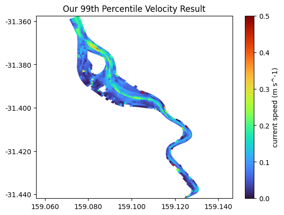
stat.plot('V_p99', cmap='turbo', clim=(0,0.5))
plt.title('Our 99th Percentile Velocity Result')
Text(0.5, 1.0, 'Our 99th Percentile Velocity Result')
Exporting new results
You can use Xarray to export results back to netcdf.
Common examples might be to load up a very large TUFLOW FV result here in Python, do some post-processing (e.g., some statistics?), or slice it to a smaller time period, and then use the to_netcdf method to export it back. Results exported in this manner will be formatted as any normal TUFLOW FV result, and can be loaded into QGIS, for example.
As an example, we can chop our result into something much smaller, like this:
fv_small = fv.isel(Time=slice(10, 20))  # Here we've used an `Xarray` native function - isel. This selected the 10th through to 19th timestep.
fv_small.to_netcdf('my_smaller_netcdf.nc')
# fv_small
This concludes the basic usage tutorial