Gallery 1: Timeseries Plots¶

This notebook provides a series of timeseries examples used in combination with the TUFLOW FV Python Toolbox (tfv) package.

import matplotlib.pyplot as plt
import numpy as np
from pathlib import Path # We'll also make use of the `pathlib` module to assist with managing file-paths, although this is entirely optional! 
import pandas as pd
import tfv.xarray
import xarray as xr  # We utilise xarray to do all the heavy lifting 

Open TUFLOW FV Model Result¶

model_folder = Path(r'..\..\data')
model_file = 'HYD_002.nc'

fv = xr.open_dataset(model_folder / model_file, decode_times=False).tfv
#fv  # Uncomment this to display the data variables

Extract Time Series Data¶

locs = {
    'P1' : (159.0758, -31.3638),
    'P2' : (159.0845,  -31.3727),
    'P3' : (159.0906,  -31.3814),
    'P4' : (159.1001,  -31.3948),
    'P5' : (159.1154,  -31.4032),
    'P6' : (159.1266,  -31.4105),
    'P7' : (159.1202,  -31.4165),
    'P8' : (159.1178,  -31.4236),
}

ts = fv.get_timeseries(['H', 'V', 'TEMP'],locs)
#ts  # Uncomment this to display the data variables

Plot Single Time Series¶

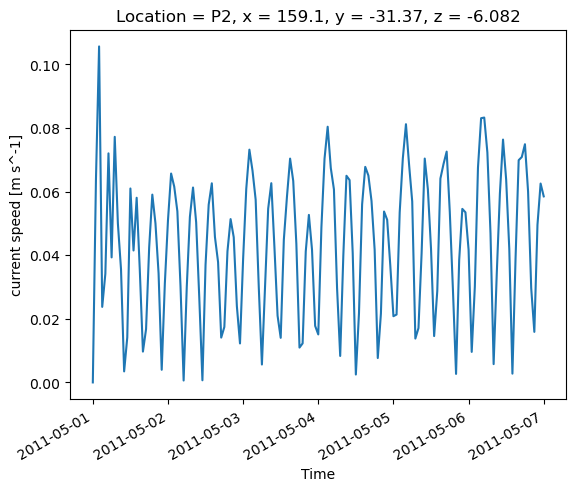
Plot the depth averaged velocity at the point P2.

ts['V'].sel(Location='P2').plot()

[<matplotlib.lines.Line2D at 0x1e3c4a3d6d0>]

../../../_images/f5cc2e061cf58e106ac8112461c2ad716204596830c64aaaeb9e4d14f65c7030.png

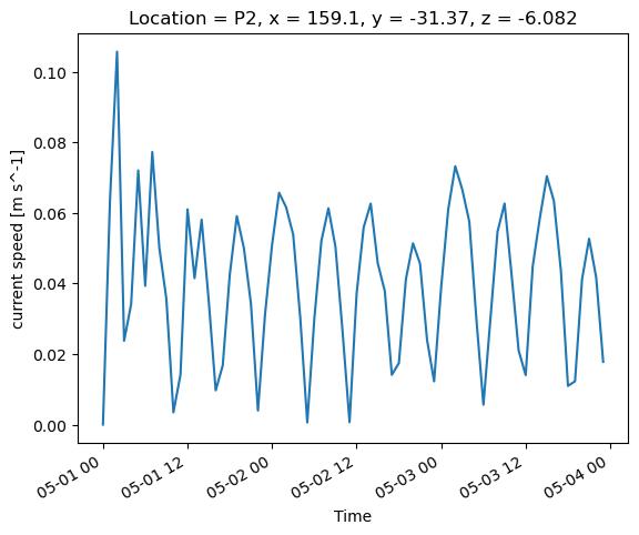
Trim the Time to Plot¶

ts['V'].sel(Time=slice('2011-05-01','2011-05-03'), Location='P2').plot()

[<matplotlib.lines.Line2D at 0x1e3c5b12850>]

../../../_images/8378eb68a80e8444edb9b71d699a39600d5770e0d6f1fabdb9b34f7cedba96e3.png

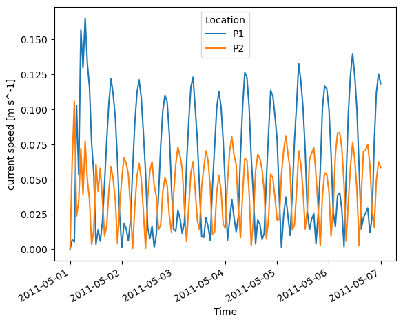
Plot Time Series at Multiple Locations¶

# Plot the time series 
ts['V'].sel(Location='P1').plot(color='red', linestyle='--')
ts['V'].sel(Location='P2').plot(color='blue')

# Tidy up the plot
plt.title('Velocity at P1 and P2')
plt.grid()
plt.ylim(0,0.2)
plt.show()

# Or you can try this for something quick
ts['V'].sel(Location=['P1','P2']).plot.line(x='Time', hue='Location')

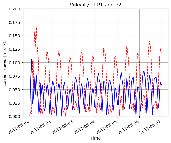
../../../_images/ae639efabc6e4cb27c3bc19685de43f389cd2dbf61a152618c41abd71155da71.png

[<matplotlib.lines.Line2D at 0x1e3c741d1d0>,
 <matplotlib.lines.Line2D at 0x1e3c741d310>]

../../../_images/2c5b081de3c6544f1d288c21925cbf29f9be8ff06bd0ce6d5ae3fee12722f67f.png

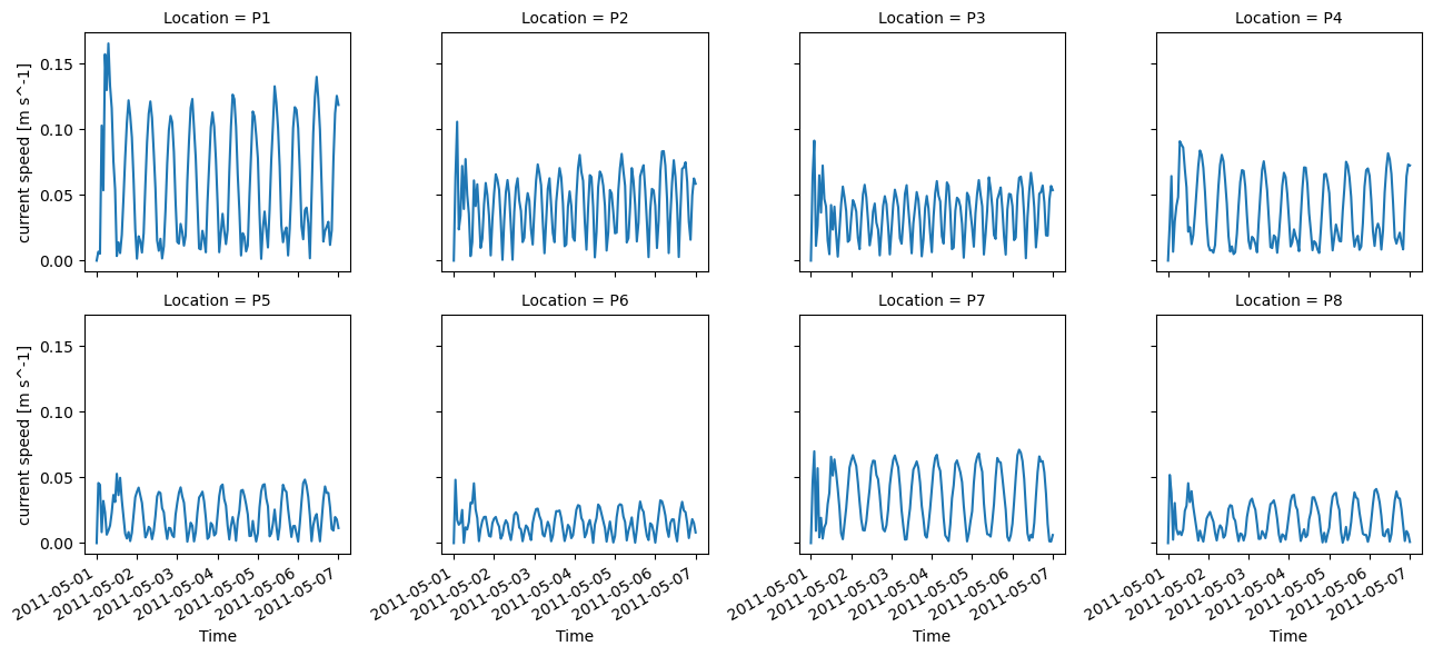
Plot Time Series at All Locations¶

ts['V'].plot.line(x='Time', col='Location',col_wrap=4)

<xarray.plot.facetgrid.FacetGrid at 0x1e3c743c980>

../../../_images/9e86dd7b93c5a5147cae6dfa08fc612304198f80a31e3ab5e87fd9c21a5d5828.png

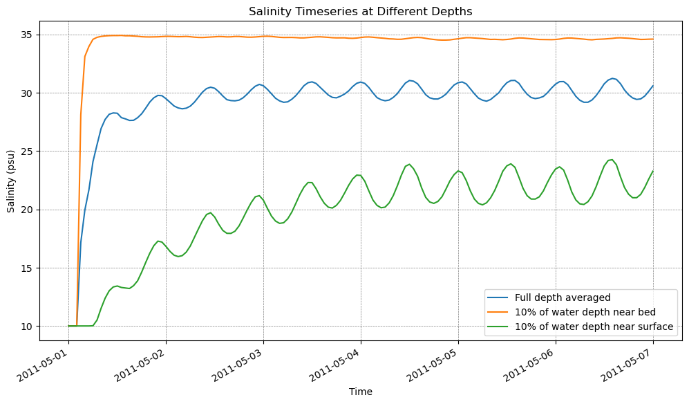
Plot Times Series at Multiple Depths and Save to Disk¶

# Extract the data at different depths (see also height, elevation and depth datum methods)
ts_dave = fv.get_timeseries(['V', 'TEMP','SAL'],locs,datum='sigma',limits=(0,1))  #   Full depth averaged
ts_bot_10pct = fv.get_timeseries(['V', 'TEMP','SAL'],locs,datum='sigma',limits=(0,0.1))  # 10% of water depth near bed
ts_top_10pct = fv.get_timeseries(['V', 'TEMP','SAL'],locs,datum='sigma',limits=(0.9,1))  # 10% of water depth near surface

# Plot the salinity timeseries in three colours on a plot
fig, ax = plt.subplots(figsize=(12,6))
ts_dave['SAL'].sel(Location='P2').plot(ax=ax, label='Full depth averaged')
ts_bot_10pct['SAL'].sel(Location='P2').plot(ax=ax, label='10% of water depth near bed')
ts_top_10pct['SAL'].sel(Location='P2').plot(ax=ax, label='10% of water depth near surface')

ax.legend()
ax.set_ylabel('Salinity (psu)')
ax.set_xlabel('Time')
ax.set_title('Salinity Timeseries at Different Depths')
ax.grid(color='grey', linestyle='--', linewidth=0.5)

plt.show()

# Save the plot to a jpg file
output_folder = Path('./outputs')
output_folder.mkdir(exist_ok=True) # Make the folder, if it doesn't exist

fig.savefig(output_folder / 'salinity_timeseries.jpg', dpi=300)

../../../_images/4cf1facf7f3d7c972c70480e31f904a82f3bdc6ecbd90947476d601f67f9dcca.png

Convert to Pandas Dataframe¶

# This example is not used further in the tutorial, but is included to show how to convert the xarray dataset to a pandas dataframe
ts_df = ts.to_dataframe()
# ts_df.head()  # Uncomment if you'd like to see a description of the pandas DataFrame

Read TUFLOW FV CSV Point Using Pandas¶

The examples shown below use Pandas to read TUFLOW FV csv POINTS output. They can be extended to read any other TUFLOW FV csv outputs such as FLUX, STRUCT_FLUX and MASS.

point_output_csv = 'HYD_002_POINTS.csv' # Output directrly from TUFLOW FV via a point output block. Contains depth averaged results at the same locations as the variable locs. 
time_format_fv_isodate = True

# Open the csv file with Pandas using the TIME column as the index and only the column we are interested in
if time_format_fv_isodate:
    df = pd.read_csv(model_folder  / point_output_csv, dayfirst=True, index_col=0, parse_dates=[0])
else:
    df = pd.read_csv(model_folder  / point_output_csv, index_col=0)

#df
df.head()

	P1_H [m]	P1_VX [m s^-1]	P1_VY [m s^-1]	P1_SAL [psu]	P1_TEMP [degrees celsius]	P2_H [m]	P2_VX [m s^-1]	P2_VY [m s^-1]	P2_SAL [psu]	P2_TEMP [degrees celsius]	...	P7_H [m]	P7_VX [m s^-1]	P7_VY [m s^-1]	P7_SAL [psu]	P7_TEMP [degrees celsius]	P8_H [m]	P8_VX [m s^-1]	P8_VY [m s^-1]	P8_SAL [psu]	P8_TEMP [degrees celsius]
TIME
2011-05-01 00:00:00	-0.010398	0.000000	0.000000	10.00000	20.00000	-0.010405	0.000000	0.000000	10.00000	20.00000	...	-0.010400	0.000000	0.000000	10.00000	20.00000	-0.010377	0.000000	0.000000	10.00000	20.00000
2011-05-01 00:15:00	0.051950	0.052889	-0.146555	10.03082	19.99511	0.048524	0.101491	-0.068855	10.00002	19.99476	...	0.003502	0.025307	0.014604	10.00003	19.99238	0.005328	-0.016296	0.025435	10.00002	19.99417
2011-05-01 00:30:00	0.033113	0.048022	-0.129686	15.16036	19.99386	0.046323	0.097354	-0.066197	10.00004	19.99046	...	0.038509	-0.017657	-0.008679	10.00006	19.98565	0.024863	0.001364	-0.002373	10.00004	19.98931
2011-05-01 00:45:00	0.013991	0.027242	-0.074837	20.79982	19.99056	0.038319	0.006228	-0.003973	10.00004	19.98816	...	0.086387	-0.074545	-0.044288	10.00011	19.96712	0.091424	0.033403	-0.052762	10.00005	19.98284
2011-05-01 01:00:00	-0.009358	-0.003516	0.003658	22.04488	19.98968	0.011016	-0.060272	0.041985	10.00004	19.98776	...	0.109613	0.045066	0.023506	10.00015	19.95416	0.122923	-0.030464	0.047189	10.00008	19.97423

5 rows × 40 columns

Plot Temperature Time Series At Single Location Using The Column Name¶

df['P1_H [m]'].plot(ylabel='Water Level [mMSL]', title='Water Level at P1')

<Axes: title={'center': 'Water Level at P1'}, xlabel='TIME', ylabel='Water Level [mMSL]'>

../../../_images/bdb39dc03885373ff10820becc8c5a53729a585a0f79760bf47881d4ca776c59.png

Temperature Time Series Plot All Locations Using Filter¶

# Plot the temperature time series at all sites where the header contains 'TEMP'
df.filter(like='TEMP').plot(ylabel='Temperature [deg C]', title='Depth Averaged Temperature at All Locations')

<Axes: title={'center': 'Depth Averaged Temperature at All Locations'}, xlabel='TIME', ylabel='Temperature [deg C]'>

../../../_images/e53b6c8233c0039cead770b05cf856fd111718f6ae2cbddcd99e1ced90eca580.png

Temperature Time Series Plot Single Location Using Filters¶

# Plot the temperature time series at all sites where the header contains 'TEMP' and Site P1
df.filter(like='TEMP').filter(like='P1').plot()

<Axes: xlabel='TIME'>

../../../_images/2daf7a33a3ffd7cbafab611839b4605a542f41e8504f37b71681edb04f18cf68.png

Plot Velocity Magnitude and Direction At Single Location¶

# Plot the velocity magnitude time series at all sites 
x_comp = df.filter(like='VX')
y_comp = df.filter(like='VY')

vmag = ((x_comp.values**2) + (y_comp.values**2))**0.5
vmag_columns = [col[:2] + '_VMAG [m s^-1]' for col in x_comp.columns]

# Cartesian direction, degrees measured anti-clockwise from due east, heading to
v_dir = np.degrees(np.arctan2(y_comp.values, x_comp.values)) % 360

# if wanting velocity direction in degrees measured anti-clockwise from due north, heading to, use the following line:
# v_dir = (90 - np.degrees(np.arctan2(y_comp.values, x_comp.values))) % 360

# if procesing wind direction in nautical convention, i.e. in degrees measured clockwise from due north,  coming from, use the following line:
# v_dir_c = (270 - np.degrees(np.arctan2(y_comp.values, x_comp.values))) % 360

v_dir_columns = [col[:2] + '_VDIR [deg]' for col in x_comp.columns]

# Add the velocity magnitude to the dataframe
df[vmag_columns] = vmag
df[v_dir_columns] = v_dir

# Setup a plot to have two horizontal subplots with shared x-axis, the top subplot for the velocity magnitude and the bottom for the velocity direction. 
fig, axes = plt.subplots(2, 1, figsize=(12, 8), sharex=True)
#df[vmag_columns].plot(ax=axs[0])
#df[v_dir_columns].plot(ax=axs[1])

# To only plot velocity at a single location P1 for example uncomment the following two lines and comment out the two plot lines immediately above this comment
df[vmag_columns].filter(like='P1').plot(ax=axes[0], color='blue')
df[v_dir_columns].filter(like='P1').plot(ax=axes[1], color='red')


# Tidy up the plot
axes[0].set_ylabel('Current Magnitude [m s^-1]')
axes[0].set_title('Current Magnitude and Direction')
axes[0].grid()
axes[0].legend(loc='upper right')
axes[0].set_ylim(0, 0.2)

axes[1].set_ylabel('Current Direction [deg cartesian convention')
axes[1].set_xlabel('Time')
axes[1].grid()
axes[1].legend(loc='upper right')
axes[1].set_ylim(0, 360)
axes[1].set_yticks(np.arange(0, 361, 60))

plt.show()

[<matplotlib.axis.YTick at 0x1e3cabe79d0>,
 <matplotlib.axis.YTick at 0x1e3c909df90>,
 <matplotlib.axis.YTick at 0x1e3c909e710>,
 <matplotlib.axis.YTick at 0x1e3c909ee90>,
 <matplotlib.axis.YTick at 0x1e3c909f610>,
 <matplotlib.axis.YTick at 0x1e3c909fd90>,
 <matplotlib.axis.YTick at 0x1e3c906ce10>]

../../../_images/1a03ba1ace0b6b2d59a0f5c29c509287e6ca0bb7502ed542712d4981fe3865c0.png

Plot Velocity Magnitude and Direction At All Locations¶

# Create 8x2 subplot grid (8 rows, 2 columns)
fig, axes = plt.subplots(nrows=8, ncols=2, figsize=(12, 24), constrained_layout=True)

# Loop through each location and plot velocity magnitude and direction
locations = [f'P{i}' for i in range(1, 9)]
for i, location in enumerate(locations):
    # Calculate row and column index for subplots
    row = i
    col1, col2 = 0, 1  # Column 1 for magnitude, column 2 for direction

    # Plot velocity magnitude
    df[f'{location}_VMAG [m s^-1]'].plot(
        ax=axes[row, col1], color='blue', label='Current Magnitude'
    )
    axes[row, col1].set_title(f'{location} - Current Magnitude')
    axes[row, col1].set_ylabel('Magnitude [m/s]')
    axes[row, col1].set_xlabel('')
    axes[row, col1].set_ylim(0, 0.2)
    
    # Plot velocity direction
    df[f'{location}_VDIR [deg]'].plot(
        ax=axes[row, col2], color='green', label='Direction (deg anti-clockwise from due east, going to)'
    )
    axes[row, col2].set_title(f'{location} - Current Direction')
    axes[row, col2].set_ylabel('Direction [deg]')
    axes[row, col2].set_xlabel('')
    axes[row, col2].set_ylim(0, 360)
    axes[row, col2].set_yticks(np.arange(0, 361, 60))

# Set x-axis labels only for the bottom plots
for ax in axes[-1, :]:
    ax.set_xlabel('TIME')
    
# Use a common legend at the bottom
fig.legend(['Velocity Magnitude', 'Direction (deg from North)'], loc='lower center', ncol=2)

plt.show()

<matplotlib.legend.Legend at 0x1e3cb6796d0>

../../../_images/2960990f15a0bd4e465842406d88a24716bd6cde6701a4ecc8e6ade0dc83f059.png

Save Data At Specific Time¶

# Return data for the time 01/05/2011 06:00:00
my_time_slice = df.loc['2011-05-01 06:00:00']

# Save the sample to a CSV file
output_folder = Path('./outputs')
output_folder.mkdir(exist_ok=True) # Make the folder, if it doesn't exist

my_time_slice.to_csv(output_folder / 'sample.csv')

# Display the data
my_time_slice

P1_H [m]                      -0.028068
P1_VX [m s^-1]                 0.044796
P1_VY [m s^-1]                -0.133019
P1_SAL [psu]                  29.443830
P1_TEMP [degrees celsius]     19.945910
P2_H [m]                      -0.021819
P2_VX [m s^-1]                 0.040056
P2_VY [m s^-1]                -0.027276
P2_SAL [psu]                  24.138690
P2_TEMP [degrees celsius]     19.941330
P3_H [m]                      -0.018699
P3_VX [m s^-1]                -0.004934
P3_VY [m s^-1]                -0.044464
P3_SAL [psu]                  21.693890
P3_TEMP [degrees celsius]     19.925860
P4_H [m]                      -0.015391
P4_VX [m s^-1]                 0.052520
P4_VY [m s^-1]                -0.011572
P4_SAL [psu]                  10.005420
P4_TEMP [degrees celsius]     19.917750
P5_H [m]                      -0.016544
P5_VX [m s^-1]                -0.000625
P5_VY [m s^-1]                -0.000521
P5_SAL [psu]                  10.000560
P5_TEMP [degrees celsius]     19.819820
P6_H [m]                      -0.017890
P6_VX [m s^-1]                 0.002982
P6_VY [m s^-1]                -0.004197
P6_SAL [psu]                  10.000420
P6_TEMP [degrees celsius]     19.858290
P7_H [m]                      -0.018583
P7_VX [m s^-1]                 0.010893
P7_VY [m s^-1]                 0.007559
P7_SAL [psu]                  10.000530
P7_TEMP [degrees celsius]     19.820050
P8_H [m]                      -0.018577
P8_VX [m s^-1]                -0.001176
P8_VY [m s^-1]                 0.001863
P8_SAL [psu]                   9.649845
P8_TEMP [degrees celsius]     19.444580
P1_VMAG [m s^-1]               0.140359
P2_VMAG [m s^-1]               0.048461
P3_VMAG [m s^-1]               0.044737
P4_VMAG [m s^-1]               0.053780
P5_VMAG [m s^-1]               0.000814
P6_VMAG [m s^-1]               0.005149
P7_VMAG [m s^-1]               0.013259
P8_VMAG [m s^-1]               0.002203
P1_VDIR [deg]                288.611633
P2_VDIR [deg]                325.747278
P3_VDIR [deg]                263.667852
P4_VDIR [deg]                347.574342
P5_VDIR [deg]                219.809159
P6_VDIR [deg]                305.394551
P7_VDIR [deg]                 34.759004
P8_VDIR [deg]                122.253055
Name: 2011-05-01 06:00:00, dtype: float64

Plot Results On A Specific Day¶

# Plot any times on a particular day
df.loc['2011-05-01'].filter(like='SAL').plot(ylabel='Salinity (psu)', title='Depth Averaged Salinity on 01/05/2011')

<Axes: title={'center': 'Depth Averaged Salinity on 01/05/2011'}, xlabel='TIME', ylabel='Salinity (psu)'>

../../../_images/dccf4068fa37caba98a9108a414bf2a6e614696bf2b59d6a0007385e22b10495.png

Plot Results Over A Specific Time Range¶

# Return and plot SAL data over the time range 01/05/2011 06:00:00 to 01/05/2011 12:00:00
df.loc['2011-05-01 06:00:00':'2011-05-01 12:00:00'].filter(like='SAL').plot(ylabel='Salinity (psu)', title='Depth Averaged Salinity')

<Axes: title={'center': 'Depth Averaged Salinity'}, xlabel='TIME', ylabel='Salinity (psu)'>

../../../_images/1f0fc44a21459be469d697c3302c02c94d74e515962f2512222384741ea770cc.png

Plot Results Over A Specific Time Range And Location¶

# Return and plot SAL data over the time range 01/05/2011 06:00:00 to 01/05/2011 12:00:00 for locations P1 and P2
df.loc['2011-05-01 06:00:00':'2011-05-01 12:00:00'].filter(like='SAL').filter(like='P1').plot(ylabel='Salinity (psu)', title='Depth Averaged Salinity at P1')

<Axes: title={'center': 'Depth Averaged Salinity at P1'}, xlabel='TIME', ylabel='Salinity (psu)'>

../../../_images/511f991ca5128d824c3fc58367257d37602ff89c6c81e4e9b8cb98d117ce7d7b.png

Combining TUFLOW FV XArray and Pandas¶

fig, ax = plt.subplots(figsize=(12,6))

# Plot the salinity timeseries in three colours on a plot
# Note: Convert xarray data to pandas Series - this avoids xarray pandas axes converter issues
ts_dave['SAL'].sel(Location='P2').to_series().plot(ax=ax, label='Full depth averaged')
ts_bot_10pct['SAL'].sel(Location='P2').to_series().plot(ax=ax, label='10% of water depth near bed')
ts_top_10pct['SAL'].sel(Location='P2').to_series().plot(ax=ax, label='10% of water depth near surface')

# Add SAL at P2 from the Pandas dataframe
df.filter(like='SAL').filter(like='P2').plot(ax=ax, color='red', linestyle='--')

# Labels and title
ax.legend()
ax.set_ylabel('Salinity (psu)')
ax.set_xlabel('Time')
ax.set_title('Salinity Timeseries at Different Depths Plus POINTS CSV Depth Average')
ax.grid(color='grey', linestyle='--', linewidth=0.5)

plt.show()

../../../_images/9353a1f4343540d414f0c9c9f02ffecdf96f3397449c2169648929c2f9b0c785.png

This concludes the examples on time series plotting.