Gallery 4: Curtain Plots

Curtain plots allow you to review 3D results along a long section or cross section.

This notebook is used in combination with the TUFLOW FV Python Toolbox (tfv) package. To follow along on your own computer, please download the demonstration notebooks from the TUFLOW Downloads Page. Look for the TUFLOW FV Python Toolbox download. Installation instructions are provided on our TUFLOW FV Python Toolbox Wiki Page.

import xarray as xr  # We utilise xarray to do all the heavy lifting 
import tfv.xarray
from pathlib import Path # We'll also make use of the `pathlib` module to assist with managing file-paths, although this is entirely optional! 
import matplotlib.pyplot as plt
import seaborn as sns
import numpy as np

Open TUFLOW FV Model Result

model_folder = Path(r'..\..\data')
model_file = 'HYD_002.nc'

fv = xr.open_dataset(model_folder / model_file, decode_times=False).tfv
#fv  # Uncomment if you would like to review the Dataset

Single Curtain Plot

from matplotlib.gridspec import GridSpec
sns.set(style='white', font_scale=0.9)

polyline = np.loadtxt(model_folder / 'polyline.csv', skiprows=1, delimiter=',')

time = '2011-05-02 12:00'
vardict = {
    'TEMP': dict(cmap='inferno', clim=(10, 22)),
    'SAL': dict(cmap='ocean', clim=(0, 36)),
    'V': dict(cmap='jet', clim=(0, 1)),
}

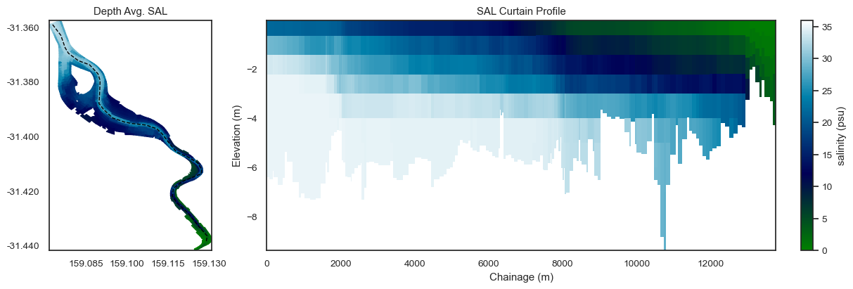
var = 'SAL'

# Create figure
fig, (ax1, ax2) = plt.subplots(1, 2, figsize=(12, 4), gridspec_kw={'width_ratios': [1, 3]}, constrained_layout=True)

cspec = vardict[var]
fv.plot(var, time, ax=ax1, colorbar=False, **cspec)
ax1.plot(polyline[:, 0], polyline[:, 1], lw=1, color='black', ls='--')
ax1.set_aspect('equal')
ax1.set_title(f'Depth Avg. {var}')

fv.plot_curtain(polyline, var, time, ax=ax2, ec='none', **cspec)
ax2.set_title(f'{var} Curtain Profile')

plt.show()

Multiple Curtain Plots

# Create figure
fig, (ax1, ax2, ax3) = plt.subplots(3, 1, figsize=(12, 8), constrained_layout=True)


var = 'SAL'
cspec = vardict[var]
fv.plot_curtain(polyline, var, time, ax=ax1, ec='none', **cspec)
ax1.set_title(f'{var} Curtain Profile')

var = 'TEMP'
cspec = vardict[var]
fv.plot_curtain(polyline, var, time, ax=ax2, ec='none', **cspec)
ax2.set_title(f'{var} Curtain Profile')

var = 'V'
cspec = vardict[var]
fv.plot_curtain(polyline, var, time, ax=ax3, ec='none', **cspec)
ax3.set_title(f'{var} Curtain Profile')

plt.show()

Plot Interactive Curtain

%matplotlib widget

fv.plot_curtain_interactive(polyline, 'SAL', cmap='turbo', clim=(10,35), edgecolor='face')
plt.ylim(-10, 2)
plt.show()

This concludes the examples on curtain plotting.